Plotting the far field
This example contains the simulation of a plane wave scattered by a spiral of fifteen glass spheres on a glass substrate under oblique incidence.
Click here
to download the Python script.
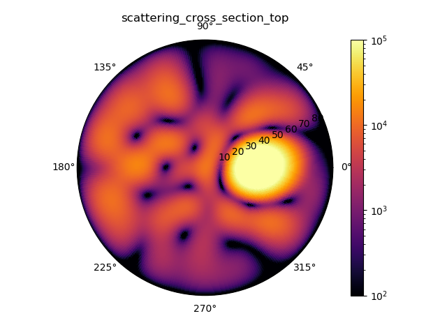
ambient DSCS |
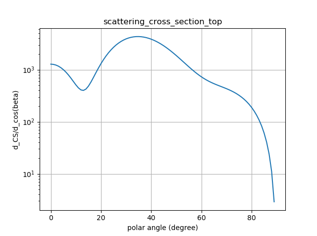
ambient DSCS (integrated over \(\alpha\)) |
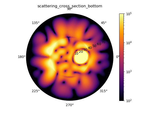
substrate DSCS |
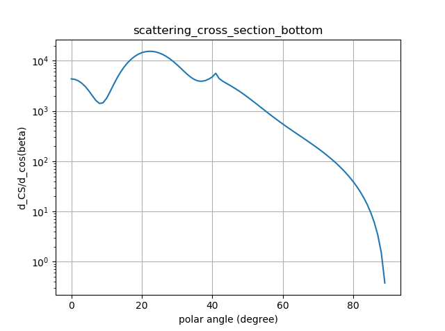
substrate DSCS (integrated over \(\alpha\)) |
After the simulation has run, the differential scattering cross section is evaluated in a post processing step. The left column shows the 2D-differential scattering cross section, \(\mathrm{DSCS}(\alpha, \beta) = \frac{\mathrm{dSCS}}{\mathrm{d}\Omega}\), whereas the right column shows the 1D distribution (i.e., the integral over the azimuthal direction coordinate), \(\mathrm{DSCS}(\beta) = \frac{\mathrm{dSCS}}{\mathrm{d}\cos\beta}\).
In the substrate far field, the critical angle is visible as a ring-shaped feature.
Click on the following link to view the API documentation of the function that is used to calculate and plot the fields.
smuthi.postprocessing.graphical_output.show_scattering_cross_section()